The propagation of TDKS state is implemented in the adiabatic basis \(\{ \phi_{i\mathbf{k}}(\mathbf{G},t_1) \}\) , which are the eigenstates of the Hamiltonian \(\mathcal{H}_\mathbf{k}( \mathbf{G},t_1)\):
 where band index \(i\) values from 1 to the number of bands \(N_b\), typically \(N_b \geq 2 N_e\) , and \(\varepsilon_{i\mathbf{k}}\) is the eigenvalue. The respective operators (e.g. Hamiltonian) represented in the PW basis and the adiabatic basis are notated as \(\mathcal{A}\) and \(\mathbf{A}\), respectively. The TDKS state \(\psi_{\gamma \mathbf{k} }( \mathbf{G},t)\) at each \(\mathbf{k}\) point can be expanded in the adiabatic basis \(\{ \phi_{i\mathbf{k}}(\mathbf{G},t_1) \}\) :
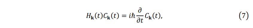
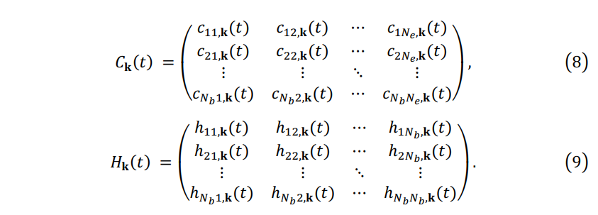
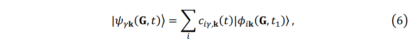 where the coefficient \(c_{i\gamma,\mathbf{k}}(t)\) is \(\left \langle \phi_{i\mathbf{k}}(\mathbf{G},t_1) | \psi_{\gamma \mathbf{k} }( \mathbf{G},t) \right \rangle\) . The Hamiltonian in the adiabatic basis \(\{ \phi_{i\mathbf{k}}(\mathbf{G},t_1) \}\) is represented by the matrix \(\mathbf{H}\) of size \(N_b\), which element is \(h_{ij,\mathbf{k}} (t)=\left \langle \phi_{i\mathbf{k}}(\mathbf{G},t_1) | \mathbf{H_k}(\mathbf{G},t) | \phi_{j\mathbf{k}}(\mathbf{G},t_1)\right \rangle\) . Thus, the TDKS equation in the adiabatic basis \(\{ \phi_{i\mathbf{k}}(\mathbf{G},t_1) \}\) is
 where
where
When \(\Delta t = t_2 - t_1 \sim 0.2\) fs, Hamiltonian in the adiabatic basis changes approximately linearly within \([t_1,t_2]\) [7, 8]:
 The matrix element of \(\mathbf{H_k}(t_1)\) in the adiabatic basis \(\{ \phi_{i\mathbf{k}}(\mathbf{G},t_1) \}\) is
 The matrix of basis change \(\mathbf{S_k}\) , an unitary matrix of size \(N_b\), can be defined as \(s_{ij,\mathbf{k}} (t_1 )=\left \langle\phi_{i\mathbf{k}}(\mathbf{G},t_2) | \phi_{j\mathbf{k}} (G,t_1 ) \right \rangle\), where \(\{ \phi_{i\mathbf{k}}(\mathbf{G},t_2) \}\) can be obtained by diagonalization of \(\mathbf{H_k}(\mathbf{G},t_2)\), like Eq. (5),
 The matrix \(\mathbf{H_k}(t_2)\) in the adiabatic basis \(\{ \phi_{i\mathbf{k}}(\mathbf{G},t_1) \}\) is represented as
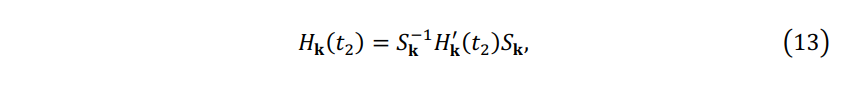 where \(\mathbf{H_k}^{'}(t_2)\) is Hamiltonian at time \(t_2\) in the adiabatic basis \(\{ \phi_{i\mathbf{k}}(\mathbf{G},t_2) \}\) , which element is \(h_{ij,\mathbf{k}}^{'} (t_2)=\left \langle \phi_{i\mathbf{k}}(\mathbf{G},t_2) | \mathbf{H_k}(\mathbf{G},t_2) | \phi_{j\mathbf{k}}(\mathbf{G},t_2)\right \rangle = \delta_{ij}\varepsilon_{i,\mathbf{k}} (t_2 )\).
The solution of Eq. (7) can be exactly written by,
 where the \(\mathbf{U_k} (t_2,t_1 )\) is evolution operator. According to Crank-Nicholson algorithm[9], when time step \(dt\) is sufficiently small and \(dt\mathbf{H} \ll 1\), the approximate expression of \(\mathbf{U_k} (t_s+dt,t_s )\) is
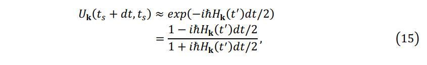 where \(t^{'} = t_s+dt/2\). Thus \(\mathbf{U_k} (t_2,t_1 )\) can be expanded as:
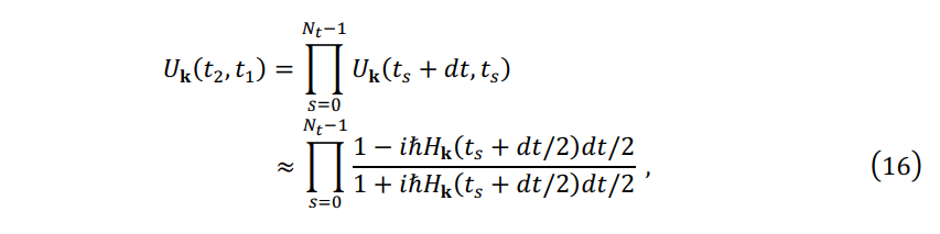 where \(t_s= t_1+sdt\), \(dt=\Delta t / N_t \sim 0.1\) attosecond, and \(\mathbf{H_k}(t_s+dt/2)\) is calculated by Eqs. (10)-(13).
Typically, the dimension of operator represented in the adiabatic basis (\(N_b \times N_b\) ), is usually much less than that in the PW basis (\(N_{\mathbf{G}} \times N_{\mathbf{G}}\) ) because \(N_b(\sim 10^2)\) is less than the number of \(\{G\}\), \(N_{\mathbf{G}}(\sim 10^4)\). Thus, it is high performance to solve the Eq. (7) in the adiabatic basis rather than the Eq. (1) in the PW basis. The computational cost mainly comes from the diagonalizing of \(\mathcal{H_k}(t_2)\) in Eq. (12).